PROBLEM
Following are the figures for the number of defectives in 22 lots each containing 2000 rubber beds:
| 425 | 430 | 216 | 341 | 225 |
| 322 | 425 | 430 | 216 | 341 |
| 225 | 322 | 280 | 306 | 337 |
| 305 | 356 | 402 | 216 | 264 |
| 126 | 409 | |||
Draw the control chart for the fraction defective, Plot the points on it. Comment on the state of control of the process.
Theory-
Control Chart for fraction defective-
We know that,
When Standard given as P = P’
Then control limits are given by-
Lower control limit,
Upper control limit,
Central Line = P’
When Standard not Given-
First we estimate the value pf P as-
Lower Control Limit,
Upper Control Limit,
Where,
A is a function of n (sample size ) and can be obtained from fraction defective chart for different value of n.
And if LCL becomes -ve than we take it as 0. Because fraction defective can’t be -ve.
R Code-
#Command To Remove Previous Objects
rm(list=ls())

#Loading Some Library
library(readxl)
library(readr)

#Loading The Given Data set And checking The Characteristics
RubberBedData=read_excel("class work 10.xlsx")
View(RubberBedData)
mode(RubberBedData)

#Creating Somr Variable
No_of_Observation=length(RubberBedData[[1]])
SampSize=2000
Sample_No=c(1:No_of_Observation)

#Calculatinf Fraction Defective In Sample
No_Of_Defective=RubberBedData[[1]]
FractionDefective=RubberBedData[[1]]/SampSize
View(data.frame(No_Of_Defective,FractionDefective))

#Estimating Population Fraction Defective And Control Charts
PooledFracDefective=sum(FractionDefective)/No_of_Observation
lcl=PooledFracDefective-3*(PooledFracDefective*(1-PooledFracDefective)/SampSize)^(0.5)
if(lcl<0){lcl=0}
LCL=lcl
UCL=PooledFracDefective+3*(PooledFracDefective*(1-PooledFracDefective)/SampSize)^(0.5)
CENTRAL_LINE= PooledFracDefective
View(data.frame(LCL, CENTRAL_LINE, UCL))

#Plotting The Process Control Graph For Mean Of Given Data
plot(Sample_No,rep(CENTRAL_LINE,No_of_Observation),type="l",ylim=c(0.05,0.3),col="black",lwd=3,ylab="Sample Fraction Defective",main="Fraction Defective Chart Of Given Data")
lines(rep(UCL,No_of_Observation),type="l",col="red",lwd=3)
lines(rep(LCL,No_of_Observation),type="l",col="yellow",lwd=3)
lines(FractionDefective,type="b",col="green",lwd=3)

#Drawing The Legend
legend("topright",legend=c(expression(bold("Upper Line = UCL")),expression(bold("Middle Line = Central Line")),expression(bold("Lower Line = LCL"))),fill=c("red","black","yellow"))
Insights From The R Console-
Obtained Sample Fraction Defective-
View(data.frame(No_Of_Defective,FractionDefective))
| S.No. | No_Of_Defective | FractionDefective |
| 1 | 425 | 0.2125 |
| 2 | 430 | 0.2150 |
| 3 | 216 | 0.1080 |
| 4 | 341 | 0.1705 |
| 5 | 225 | 0.1125 |
| 6 | 322 | 0.1610 |
| 7 | 425 | 0.2125 |
| 8 | 430 | 0.2150 |
| 9 | 216 | 0.1080 |
| 10 | 341 | 0.1705 |
| 11 | 225 | 0.1125 |
| 12 | 322 | 0.1610 |
| 13 | 280 | 0.1400 |
| 14 | 306 | 0.1530 |
| 15 | 337 | 0.1685 |
| 16 | 305 | 0.1525 |
| 17 | 356 | 0.1780 |
| 18 | 402 | 0.2010 |
| 19 | 216 | 0.1080 |
| 20 | 264 | 0.1320 |
| 21 | 126 | 0.0630 |
| 22 | 409 | 0.2045 |
Obtained LCL, Central Line And UCL-
View(data.frame(LCL, CENTRAL_LINE, UCL))
| S.No. | LCL | CENTRAL_LINE | UCL |
| 1 | 0.1328297 | 0.15725 | 0.1816703 |
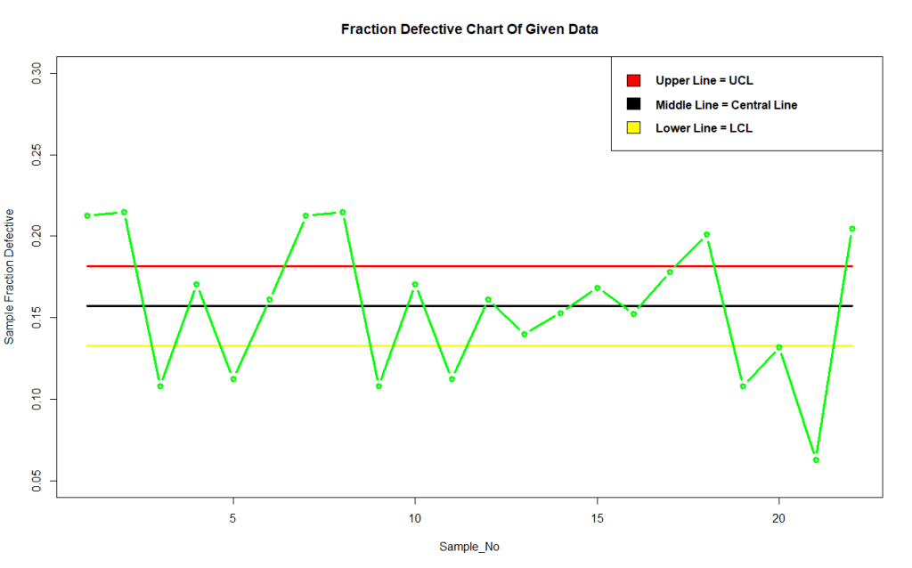
Obtained Fraction Defective Control Chart-
#Plotting The Process Control Graph For Mean Of Given Data
plot(Sample_No,rep(CENTRAL_LINE,No_of_Observation),type="l",ylim=c(0.05,0.3),col="black",lwd=3,ylab="Sample Fraction Defective",main="Fraction Defective Chart Of Given Data")
lines(rep(UCL,No_of_Observation),type="l",col="red",lwd=3)
lines(rep(LCL,No_of_Observation),type="l",col="yellow",lwd=3)
lines(FractionDefective,type="b",col="green",lwd=3)

#Drawing The Legend
legend("topright",legend=c(expression(bold("Upper Line = UCL")),expression(bold("Middle Line = Central Line")),expression(bold("Lower Line = LCL"))),fill=c("red","black","yellow"))

Conclusion-
In the above chart, we observe that many points are lying outside the control limits. Hence we conclude that the process is completely out of control.
Want To See Practically?
- download problem dataset.
- Copy-paste the R Code on RStudio.
- Goto, RStudio > Session > Set Working Directory > Choose Working Directory > “Open the folder where you downloaded the Problem dataset”
- Select The R Code > Run…That’s it 🙂